Group Equivariant Neural Networks
This webpage consists of a set of notes we created while studying the course An Introduction to Group Equivariant Deep Learning by Erik Bekkers at the University of Amsterdam. The course materials are freely available online at uvagedl, and the lecture series is available as a public playlist on YouTube. We owe our deepest gratitude for Dr. Erik Bekkers and all other people who created this wonderful course and made the materials publically available. We largely follow the structure of these lectures, even though some of the mathematical details are our own takes on the original arguments. The intrigued reader is highly recommended to check out the original lectures, where concepts are illustrated with many amazing graphics. We hope to duely justify the slogan 'Group convolution is all you need' through this short digest.
Picture credit: Dr. Bernd Frassek
Introduction
Convolutional Neural Networks (CNNs) possess the distinguishing property of translation invariance in their convolutional layers, allowing them to maintain the inherent spatial structure of image data. This characteristic enables CNNs to excel in various complex tasks, including edge detection, feature extraction for object recognition, and semantic segmentation.
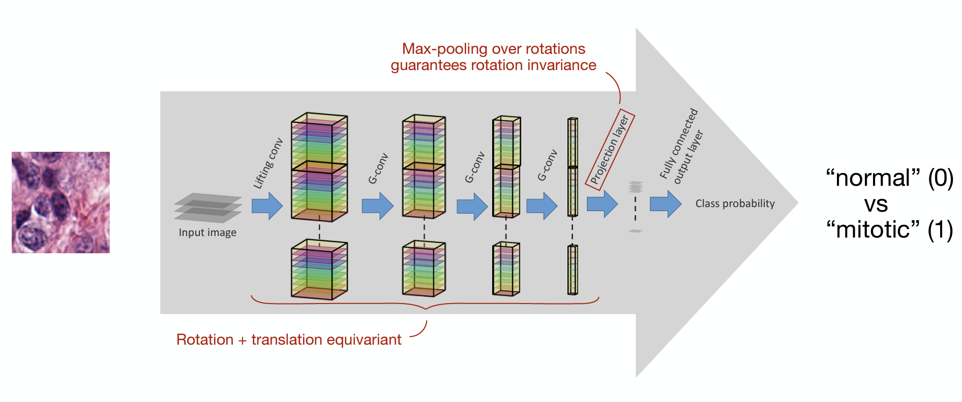
However, image data often come with additional structures, such as rotational or reflectional symmetries, which are not built-in symmetries of traditional CNNs. Group-equivariant CNNs (\(G\)-CNNs) extend the translation-invariance property of traditional CNNs into equivariance of more general symmetry groups, such as rotations, reflections, or scaling transformations. This is achieved by defining convolutional layers over topological groups rather than the usual vector space \(\mathbb{R}^n\). As a result, \(G\)-CNNs efficiently represents and processes data with a lot of symmetries, in many cases improving the performance margin significantly. One of the first applications where \(G\)-CNNs are extremely useful is medical imaging, where cells and organs can appear in various orientations ([Bekkers et.al. 2018]).
!!!TBA
\(G\)-CNN: The First Class
Say we want to build a network which recognizes the letter \(G\). Regardless of where we position the \(G\) in our input image, we want the feature map of the network to activate in the same way where it detects the \(G\) somewhere in the image. This sort of translation equivariance is a defining feature of Convolutional Neural Networks (CNNs), and in fact what makes it so useful in pattern recognition tasks, especially in image and spatial data.
Convolutional Neural Networks
CNNs achieve translation invariance through the structure of their convolutional layers. Mathematically, a convolutional layer takes in a signal \(f:\mathbb{R}^n\to \mathbb{R}\) and computes a feature map \(\hat{f}(x)\) as
\[\hat{f}(x):=(\kappa * f)(x) = \int_{y\in\mathbb{R}^n} \kappa(x-y) f(y) \, dy\], where \(\kappa\) is the convolution kernel (aka. filter). If the signal \(f\) is translated by a vector \(t \in \mathbb{R}^n\), say \(f^\prime(x) = f(x + t)\), then the resulting feature map shifts correspondingly:
\[\begin{aligned} \hat{f}^\prime(x) & = (\kappa * f')(x) \\ & = \int_{\mathbb{R}^n}\kappa(x-y)f(y+t)dy \\& = \int_{\mathbb{R}^n}\kappa((x-t)-y)f(y)dy \\& = \hat{f}(x-t). \end{aligned}\]This can be organized into a commutative diagram:
\[\begin{tikzcd} f & {\hat{f}} \\ {f^\prime} & {\hat{f}^\prime} \arrow["{\tiny{\text{ convolution }}}"{marking, allow upside down}, from=1-1, to=1-2] \arrow["{\tiny{\text{ translation }}}"{marking, allow upside down}, from=1-1, to=2-1] \arrow["{\tiny{\text{ translation }}}"{marking, allow upside down}, from=1-2, to=2-2] \arrow["{\tiny{\text{ convolution }}}"{marking, allow upside down}, from=2-1, to=2-2] \end{tikzcd}\]In plain words, convolving first and then translating results the same as translating first and then convolving. This demonstrates that the convolution operation is compatible with translational symmetries and is exactly what makes CNNs so good with acoustic and visual signals.
Group Equivariant CNNs
Our physical world is brimming with symmetries – from the discrete polytopal symmetries of a virus to the rotational symmetries of the surface of a planet.
TODO: add pictures of the icosahedral and SO(3) groups
It is an inevitable consequence that the data inputted in neural networks come with a lot of built-in symmetries. Respecting, or better, leveraging those symmetries has proven to be the key in speeding up training and improving accuracy. It is therefore requisite that we build network architectures that are compatible with more general symmetries, i.e. groups other than \(\mathbb R^n\).
To do this, we ask the generalized convolution layers to satisfy a similar property:
Group convolution followed by group translation should be the same as group translation followed by group convolution.
\[\begin{tikzcd} f & {\hat{f}} \\ {f^\prime} & {\hat{f}^\prime} \arrow["{\tiny{G-\text{ convolution }}}"{marking, allow upside down}, from=1-1, to=1-2] \arrow["{\tiny{G-\text{ translation }}}"{marking, allow upside down}, from=1-1, to=2-1] \arrow["{\tiny{G-\text{ translation }}}"{marking, allow upside down}, from=1-2, to=2-2] \arrow["{\tiny{G-\text{ convolution }}}"{marking, allow upside down}, from=2-1, to=2-2] \end{tikzcd}\]Fix the ground field to be \(\mathbb k\), which for all practical purposes will be \(\mathbb R\) or \(\mathbb C\). (It will be awesome if you are able to come up with an application of \(G\)-CNNs with a more exotic ground field!)
So say we are given a function (aka. a signal) \(f\) on some space \(X\) with a large group of symmetries \(G\) –– so large that \(X\) is in fact a homogeneous space of \(G\). (This requirement is so that we have a nice representation theory of \(G\) on the space of functions over \(X\).) A \(G\)-convolution then amounts to a choice of convolution kernel \(\kappa: X \to \mathbb k\) satisfying a certain symmetry constraint, so that the convolution is \(G\)-equivariant.
Formally, assume \(X \cong G/H\) for a normal subgroup \(H\), with Haar measure \(d\mu\). We fix a representation \(\rho\) of \(G\) on the space of square-integrable functions \(L_2(X)\),with inner product denoted \(\langle -,-\rangle_X\). For a point \(x \in X\), pick a coset representative \(g_x\in G\) such that \(x = [g_xH]\). Then, a \(G\)-convolution \(\mathcal{K}: L_2(X) \to L_2(X)\) has the form
\[(\mathcal{K}f)(x) := \langle \rho(g_x)(\kappa),f\rangle_X = \int_X (g_x\cdot \kappa)fd\mu.\]In fact, it is a theorem of Bekkers that all such equivariant transformations on signals come in the form of a \(G\)-convolution!
This comes with a caviat that the kernel \(\kappa\) must be invariant under the subgroup \(H\), since we made a choice of the representative \(g_x\). Fortunately, we can choose to not worry about this constraint by lifting the convolution to the big group \(G\).
Given such, the general architecture of a \(G\)-CNN is as follows:
Start with an input signal on \(X\).
Lift the input signal to \(G\).
Convolution layer: \(G\)-convolve with a chosen kernel \(\kappa\).
Activation layer: filter the transformed signal through a chosen \(G\)-equivariant activation function.
Repeat steps 3 and 4.
Project down to \(X\) by max pooling over \(H\).


// Image matching '/assets/posts/post4/post4 assets/G-CNN-architecture.png' not found. //
In the next sections, we are going to build up the necessary representation theory and investigate how such \(G\)-convolution layers can be built computationally.
Representation Theory and Harmonic Analysis on Lie Groups
Semi-direct Products
Say we have two groups \(G\), \(H\), and we want to build a bigger group with \(G\) and \(H\) as the coordinate axes. The easiest way to do this is the direct product \(G\times H\). The next simplest thing is a "twisted product" – a semi-direct product \(G \rtimes H\).
Formally, we require an action \(\rho\) of \(H\) on \(G\). Then, as a set, the semidirect product \(G\rtimes_\rho H\) has the same elements \((g,h)\) as the direct product \(G\times H\), however with an altered group law. Namely, we define a new group product
\[(g_1, h_1)\ast (g_2,h_2):= (g_1\rho_{h_1}(g_2), h_1h_2),\]so we see that the \(G\)-coordinate has been "twisted" by the action of \(H\).
If the action \(\rho\) is trivial, then we recover the direct product of the two groups. Furthermore, we can classify all possible semidirect products in terms of non-isomorphic actions of \(H\) on \(G\). We call semidirect products a (split) extension of \(G\) by \(H\), in the sense that the groups fit into a short exact sequence
\[1\to G \to G\rtimes H \to H\to 1\]which splits – resembling a locally trivial bundle in manifold theory.
The special Euclidean group \(SE(2)\) is an extension of the group of translations \((\mathbb R^2, +)\) of the plane by rotations \(SO(2)\) in the plane. It has matrix representation
\[ g=\left(x, R_\theta\right) \quad \leftrightarrow \quad G=\left(\begin{array}{ccc} \cos \theta & -\sin \theta & x \\ \sin \theta & \cos \theta & y \\ 0 & 0 & 1 \end{array}\right)=\left(\begin{array}{cc} R_\theta & x \\ 0^T & 1 \end{array}\right) \]and group law
\[ (x, \theta) \cdot\left(x^{\prime}, \theta^{\prime}\right)=\left(R_\theta x^{\prime}+x, \theta+\theta^{\prime} \bmod 2 \pi\right) \]or in matrix form,
\[ \left(\begin{array}{cc} R_\theta & x \\ 0^T & 1 \end{array}\right)\left(\begin{array}{cc} R_\theta^{\prime} & x^{\prime} \\ 0^T & 1 \end{array}\right)=\left(\begin{array}{cc} R_{\theta+\theta^{\prime}} & R_\theta x^{\prime}+x \\ 0^T & 1 \end{array}\right). \]The Euclidean group \(E(n)\) and special Euclidean group \(SE(n)\) are similarly defined.
TODO: picture of SE2
The scale-translation group \(\mathbb R^2 \rtimes \mathbb R^\times_+\) is an extension of \(\mathbb R^2\) by the multiplicative group \(\mathbb R^\times_+\). The group law is given by
\[ g \cdot g^{\prime}=(x, s) \cdot\left(x^{\prime}, s^{\prime}\right)=\left(s x^{\prime}+x, s s^{\prime}\right) \]Lie Groups and Homogeneous Spaces
A Lie group is a topological group endowed with the structure of a smooth manifold. A transitive group action is an action with a single orbit. A homogeneous space for a Lie group \(G\) is then a smooth manifold \(X\) with a transitive \(G\)-action.
Say we have a \(G\)-action on \(X\) with just a single orbit. Then, for any point \(x\) in the single orbit \(X\), the orbit-stabilizer theorem says that
\[X = G/\mathrm{Stab}_x\]as a set, which can be upgraded to a diffeomorphism of smooth manifolds. Therefore, \(G\)-homogeneous spaces are in 1-to-1 correspondence to quotients \(G/H\) where \(H\) is a normal subgroup. Elements in \(X\cong G/H\) are then cosets of \(H\). The stabilizer subgroup \(\mathrm{Stab}_x\) is often called the isotropy subgroup of a point \(x\), which consists of all transformations in \(G\) that fix \(x\).
Any Lie group \(G\) is a homogeneous space over itself with trivial isotropy.
\[G\cong G/\{1\}.\]The orthonogal group \(O(n+1,\mathbb R)\) acts on the \(n\)-sphere \(S^n \subseteq \mathbb R^{n+1}\) with isotropy \(O(n,\mathbb R)\). Therefore,
\[S^n \cong O(n+1,\mathbb R)/O(n,\mathbb R).\]There is a similar story for the complex \((2n-1)\)-sphere in \(\mathbb C^n\).
The special Euclidean group \(SE(n)\) acts on \(\mathbb R^n\) via all rigid body motions (composites of rotations and translations). The isotropy of each point is \(SO(n)\), since a point in \(\mathbb R^n\) does not carry the data of an orientation. Therefore,
\[\mathbb R^n \cong SE(n)/SO(n).\]The group of scaling-translations \(\mathbb R^n\rtimes\mathbb R^\times_+\) acts on \(\mathbb R^n\) composites of translations and scalings. The isotropy of each point is \(\mathbb R^\times_+\), since a point in \(\mathbb R^n\) does not see the scaling. Therefore,
\[\mathbb R^n \cong (\mathbb R^n\rtimes\mathbb R^\times_+)/\mathbb R^\times_+.\]The orthonogal group \(O(n,\mathbb R)\) acts on the Grassmannian \(Gr_\mathbb R(k,n)\) of \(k\)-planes in \(n\)-space via rotating a \(k\)-plane. The isotropy of each \(k\)-plane is \(O(k)\times O(n-k)\), since each \(k\)-plane is invariant under orthogonal transformations on itself and its orthogonal complement. Therefore,
\[Gr_\mathbb R(k,n)\cong O(n)/O(k)\times O(n-k).\]There is a similar story for the complex Grassmannian \(Gr_\mathbb C(k,n)\) and for more general fields \(\mathbb k\).
Integration on Lie Groups and Homogeneous Spaces
Integration on a manifold is a pairing between formal sums of \(k\)-dimensional submanifolds and differential \(k\)-forms, which returns a scalar in \(\mathbb k = \mathbb R or \mathbb C\).
\[\text{ integral } = \int_{\text{ sum of submanifolds } C} \text{ differential form }d\mu.\]For integration over groups (and similarly homogeneous spaces), we want the number we get to be invariant if we translate our submanifold by any group element \(g\). This leads to the notion of a left-invariant measure (resp. right-invariant if the group acts on the right).
Haar measure
Given a \(G\)-space \(X\), a Borel measure \(\mu\) is left-invariant if for any subset \(C\subseteq X\) and any group element \(g\), we have \(\mu(g\cdot C) = \mu(C)\). Such a measure on \(G\) itself is called the Haar measure, whose existence and uniqueness are always guaranteed:
The idea behind the construction of Haar measures is to normalize by the scaling factor of group translations. Here are some examples.
Consider the Lie group \(\mathbb R^\times_+\) with the Euclidean topology. Consider the Lebesgue measure \(\lambda\) (\(dx\) in differential notation). Every \(x \in \mathbb R^\times_+\) acts on a subset \(C\subseteq \mathbb R^\times_+\) and stretches the volume (length since 1-dimensional) by a factor of \(x\):
\[\lambda{x\cdot C} = x\lambda(C)\]. Therefore, if we normalize \(dx\) by \(\frac{1}{x}\), then it becomes \(\mathbb R^\times_+\)-invariant. The Haar measure is therefore
\[\frac{1}{x}dx.\]This turns out to be a brilliant mnemonic for the definition of the Gamma function, where
\[\Gamma(t) = \int_{\mathbb R_+}e^{-s}s^{t-1}dt = \int_{\mathbb R_+}e^{-s}s^{t}\; \frac{1}{t}dt\]and this is really an integral over the group \(\mathbb R^\times_+\).
Any invertible matrix \(X\) in the general linear group \(GL_n(\mathbb k), \mathbb k = \mathbb R \text{ or }\mathbb C\) streches volume of \(\mathbb R^{n\times n}\) by \(|\det X|^n\). Therefore, the Haar measure is
\[\frac{1}{|\det X|^n}dX.\]The left-invariance can be an important point, since a group can have left- and right-invariant measure not agreeing up to scaling. For example, the group of matrices of the form
\[\begin{pmatrix} x & y \\ 0 & 1\end{pmatrix}\]with \(x>0\) has left-invariant measure \(\frac{1}{x^2}dxdy\) and right-invariant measure \(\frac{1}{x}dxdy\), and they are obviously different.
Left and right-invariant measures agree for unimodular groups, which includes all of compact, discrete,abelian, connected and semisimple, connected and reductive, connected and nilpotent. BerkeleyNotes offers a very nice exposition.
The Peter-Weyl Theorem and Harmonics
Now, for a homogeneous space \(X \cong G/H\), existence of the Haar measure is a bit more tricky, since it depends on something called the modular function of the Lie group \(G\) and its restriction to \(H\). Fortunately, all \(X\) in our consideration admits a unique Haar measure, say \(d\mu\), which we may use to define an (Hermitian) inner product on the space of \(\mathbb R\) (resp. \(\mathbb C\))-valued functions by setting
\[\langle f, g\rangle_X:= \int_X fgd\mu.\](The \(g\) needs conjugation for the case \(\mathbb k = \mathbb C\).) With that comes a notion of the \(L_2\) norm and the space \(L_2(X)\), i.e. the Hilbert space of square integrable functions.
Since \(G\) acts on \(X\), this action naturally extends to an action on \(L_2(X)\) where \(g\) acts by transforming the domain of \(f\in L_2(X)\). More precisely, we have the left-regular representation \(\mathcal{L}\) of \(G\) on \(L_2(X)\), where \(g\) operates by
\[g\cdot f(x) := f(g^{-1}x).\]We take put inverse of \(g\) so as to make this a left-action. Verify this on your own!
The left-regular representation is particularly important because it is faithful (respects all symmetries from \(G\)) and unitary (respects the inner product). In fact, it is a fundamental result in harnomic analysis that such unitary representations on spaces of functions completely decomposes into spaces of harmonics. This is the famous Peter-Weyl Theorem, aka. Maschke's theorem for harmonic analysts.
Basis elements for each of the irreducible pieces are called harmonics, and the term is justified through the following examples.
Let \(G = U(1)\cong SO(2)\cong S^1\). Then,
\[L_2(G) = \bigoplus_{k\in \mathbb{Z}} \mathbb C \cdot Y_k, \quad Y_k(\theta) = e^{i\theta/k}.\]This captures the familiar Fourier transform between \(S^1\) and its group of complex characters \(\mathbb{Z}\) (aka. frequencies), and the basis functions \(Y_k(\theta) = e^{i\theta/k}\) are the circular harmonics. Taking the real and imaginary parts, we recover the familiar \(\cos\) and \(\sin\) bases for Fourier series.
The circular harmonis are called steerable in the deep learning literature because they can be "steered" under rotations from \(S^1\), and the action of \(S^1\) on a signal \(f\in L_2(S^1)\) decomposes into steering circular harmonics at different frequencies.
TODO: add circular harmonics picture.
Let \(X = S^2 \cong SO(3)/SO(2)\) be the \(2\)-sphere, with affine coordinates \((\theta, \varphi)\). \(S^2\) has Haar measure \(\sin(\theta)d\varphi d\theta\). Then, we have the decomposition
\[L_2(S^2) = \bigoplus_{l \in \mathbb{N}}\bigoplus_{m = -l}^l \mathbb C\cdot Y_l^m\]where
\[Y_l^m(\theta, \varphi) = (-1)^m \sqrt{\frac{(2 \ell+1)}{4 \pi} \frac{(\ell-m)!}{(\ell+m)!}} P_{\ell}^m(\cos \theta) e^{i m \varphi}\]are the famous spherical harmonics. The \(P_l^m\) are the Legendre polynomials. Every signal \(f\in L_2(S^2)\) is then a sum of spherical harmonics, and the left-regular representation decomposes into rotating each basis harmonic in 3-space.
In fact, the spherical harmonics correspond to the famous electron orbits.
TODO: add spherical harmonics electron orbit picture.
The orthogonal basis for \(L_2(X)\) obtained via Peter-Weyl is often referred to as the steerable basis in the literature.
\(G\)-Convolutions and Architecture of \(G\)-CNNs
Say \(X \cong G/H\) for a normal subgroup \(H\), with Haar measure \(d\mu\). We fix a representation \(\rho\) of \(G\) on \(L_2(X)\) with inner product \(\langle -,-\rangle_X\). For a point \(x \in X\), pick a coset representative \(g_x\in G\) such that \(x = [g_xH]\). Then, the \(G\)-convolution \(\mathcal{K}_\rho: L_2(X) \to L_2(X)\) is defined as
\[(\mathcal{K}_\rho f)(x) := \langle \rho(g_x)(\kappa),f\rangle_X = \int_X (g_x\cdot \kappa)fd\mu.\]More generally, if \(X\cong G/H_1\) and \(Y \cong G/H_2\) are homogeneous spaces of \(G\), then for any \(y\in Y\), pick coset representative \(g_y\) such that \(y = [g_yH_2]\). The \(G\)-convolution \(\mathcal{K}: L_2(X)\to L_2(Y)\) is then
\[(\mathcal{K}_\rho f)(y) := \langle \rho(g_y)(\kappa),f\rangle_X = \int_X (g_y\cdot \kappa)fd\mu.\]Homework: verify that \(G\)-convolutions are indeed equivariant!
The usual convolution
\[\kappa\ast f(x) = \int_{y\in\mathbb R^n}\kappa(x-y)f(y)dy\]is in fact a group convolution where \(G = \mathbb R^n\) itself. The term \(-y\) in the argument of \(\kappa\) is precisely the left-regular representation \(\mathcal{L}_y\), where \(y\) acts on \(x\in R^n\) by its inverse \(-y\)!
The most important examples for us will be the left-regular representation \(\mathcal{L}\) and convolutions going between \(L_2(X)\to L_2(X)\), \(L_2(X)\to L_2(G),\) and \(L_2(G)\to L_2(X)\), as we will see in a moment.
We remember that our goal is to build convolutional layers that are equivariant under group translations. Namely, we would like to find equivariant transformations \(\mathcal{K}: L_2(X)\to L_2(Y)\). This is the content of Bekkers ICLR 2020, Thm. 1:
Let \(\mathcal{K}: L_2(X) \rightarrow L_2(Y)\) map between signals on homogeneous spaces of \(G\). Let homogeneous space \(Y \cong G / H_2\) such that \(H_2=\operatorname{Stab}_G\left(y_0\right)\) for some chosen origin \(y_0 \in Y\) and let \(g_y \in G\) such that \(\forall_{y \in Y}: y=g_y y_0\). Fix the left-regular representations on \(L_2(X)\) and \(L_2(Y)\).
Then \(\mathcal{K}\) is equivariant to group \(G\) if and only if:
It is a group convolution \(\mathcal{K}[\kappa]\): \((\mathcal{K} f)(y)=\int_X \kappa\left(g_y^{-1} x\right) f(x) \mathrm{d}\mu(x)\).
The kernel is \(H_2\)-invariant: \(\kappa(h^{-1} x)=\kappa(x)\) for all \(h\in H_2\).
TODO: add proof
Furthermore, let the big group \(G \cong X\rtimes H\) be a semidirect product and \(X = Y \cong G/H\). Any such \(H\)-invariant kernel \(\kappa\) comes from a lift \(\hat{\kappa}\in L_2(G)\) on the big group, without additional symmetry constraints.
Let \(X,G\) be as above, and \(\kappa\in L_2(X)\) be \(H\)-invariant: \(\kappa(h^{-1} x)=\kappa(x)\) for all \(h\in H\). Then, there is another kernel \(\hat{\kappa}\in L_2(G)\) and convolutions \(\mathcal{K}_{X\to G}: L_2(X)\to L_2(G)\), \(\mathcal{K}_{G\to X}:L_2(G)\to L_2(X)\) such that
\[\mathcal{K}[\kappa] = \mathcal{K}_{G\to X}\circ \mathcal{K}[\hat{\kappa}]\circ \mathcal{K}_{X\to G}.\]Conversely, any kernel \(\hat{\kappa}\in L_2(G)\) gives rise to an \(H\)-invariant kernel \(\kappa\) via the same process.
The convolution \(\mathcal{K}_{X\to G}\) is called the lifting convolution, which takes in a signal \(f\in L_2(X)\) and outputs
\[\hat{f} := \mathcal{K}_{X\to G}[\kappa](f) \in L_2(G), \quad \hat{f}(x, h) = \int_{y \in X}\kappa(h^{-1}(y-x))f(y)d\mu(y).\]The convolution \(\mathcal{K}_{G\to X}\) is given by mean pooling over \(H\).
This concludes the scaffolding of our \(G\)-CNN architecture. Since the group \(G\) for all practical purposes will be a semidirect product of \(\mathbb R^n\) with some of its symmetries, our convolutional layers can always be decomposed into a lifting convolution from \(\mathbb R^n\) to \(G\), followed by an unconstrained convolution on \(G\), followed by a pooling convolution from \(G\) back to \(\mathbb R^n\). Since we used left-regular representations throughout, such an architecture is called a regular \(G\)-convolutional network.
\(G\)-CNN: Regular v.s. Steerable Networks
So we need to lift any signal \(f\) on \(X\) (usually \(X = \mathbb R^n\)) to a signal on the big group \(G\), and this is done via the lifting convolution, where we lift the kernel \(\kappa\) to \(\hat{\kappa}\in L_2(G)\). This theoretically gives us true \(G\)-equivariance and replicates every signal to infinite precision. However, as with any other computer program, we need to choose a suitable discretization scheme.
TODO: add schematic of lifting convolution
Schematically, we have infinitely many copies of \(X\) in \(G = X\rtimes H\) indexed by \(H\), represented as the horizontal planes. These are the sections of \(X\) in \(G\). If we fix one such horizontal plane, then we see that there is a copy of \(H\) sticking out vertically of each point on the plane. These copies of \(H\) are called the fibers of the projection map \(G\to X\). It is then a question of whether to discritize horizontally or vertically.
Regular \(G\)-CNNs
Say we want to slice a feature map on \(G\) by horizontal sections. Then, each horizontal slice is just a feature map on \(X\) itself, and traversing vertically through different copies of \(X\) amounts to transforming \(X\) under the action of \(H\). For example, if we slice up a kernel \(\hat{\kappa}\) on \(SE(n)\), then each slice \(\kappa\) is just a kernel on \(\mathbb R^n\) rotated from some original position by a rotation in \(SO(n)\). Discretizing in this direction then amounts to choosing finitely many transformations in \(H\) to approximate all of \(H\).
The regular \(G\)-CNN architecture loses true equivariance, because the kernel is not transformed via all elements in \(H\). This approach resembles the traditional method of data augmentation, where the input signal is transformed by a discrete subgroup of \(H\) and then all fed into a non-equivariant convolutonal layer. The fundamental improvement here is that regular \(G\)-CNNs are able to capture local transformations because the kernel is transformed, while data augmentation methods only captures global transformations.
TODO: add schematic of local vs. global.
Steerable \(G\)-CNNs
So let's try slicing feature maps the other way, by vertical fibers. Then, the feature map remains on \(X\) but its values are signals on the fibers \(H\) over each point \(x\in X\). (This is essentially the idea of currying.)
Formally, given some signal \(f\in L_2(G)\), we view it as a two-variable function \(f(x,h)\) for \(x\in X, h\in H\) and curry it:
\[f_x: = f(x, -): H\to \mathbb R \quad \text{ for each fixed } x\in X.\]We have an "augmented" feature map
\[F: X \to L_2(H), \quad x\mapsto f_x,\]and Peter-Weyl comes in handy: we may decompose each signal on \(H\) as a sum of the \(H\)-harmonics, and discretizing this signal amounts to choosing a finite bandwidth (i.e. storing the Fourier coefficients in front of a finite number of frequencies. Since we are decomposing the fiber-wise signals into the steerable \(H\)-basis, this architecture is referred to as steerable \(G\)-CNN.
For \(G = SE(2)\), we get a feature map on \(\mathbb R^2\) of Fourier coefficients in front of the cicular harmonics.
For \(G = SE(3)\), we get a feature map on \(\mathbb R^3\) of Fourier coefficients in front of the spherical harmonics. This is essentially the content of the paper Esteves ECCV 2018.
TODO: add screenshots from the papers.
The steerable architecture achieves true equivariance, but the choice of bandwidth limits the amount of precision that the feature map is able to approximate a signal. As with Taylor and Fourier series, we can always raise the precision by choosing a bigger bandwidth (allowing more basis harmonics in the finite sum approximation).
\(G\)-Activation Layers
Finally, there is the issue that activation layers do not yet have built-in equivariance. Again, there are two approaches to build equivariant activation layers.
First, we may simply choose equivariant activation functions.
The more preferable choice is adhering to the steerable framework and apply activation functions fiber-wise. Since the signals on each fiber \(H\) is steerable, it remains steerable even if we cut off a portion of if by say a RELU. This allows basically any familiar non-linear activation function but can create sharp corners which requires a bigger bandwidth to approximate.
TODO: add steerable RELU picture
References
Prof. Jean Gallier at Penn has published a number of amazing volumes on all of the representation theory, differential geometry, and harmonic analysis useful for the above discussions. The ones particularly relevant are:
Aspects of Representation Theory and Noncommutative Harmonic Analysis
Geometric Methods and Applications For Computer Science and Engineering
Differential Geometry and Lie Groups: A Second Course
The author of this blog owes immense gratitude to Prof. Gallier for introducing him to this subject during his undergraduate and offering incredibly helpful advice.
Chen Cai has created a great repository of papers on equivariant networks: Awesome Equivariant Network.
See Geometric Deep Learning for a comprehensive treatment of geometric methods used in deep learning.